Mathematical Concepts Of Data Science

Basic overview of the Probability and Statistics you’d need on your journey to become a world-class Data Scientist.

Probability and Statistics are the quintessential foundations for everyone taking his/her first steps into Data Science. It would certainly not be wrong to say that the journey of mastering Data Science begins with Probability and Statistics.

Probability

Life is full of uncertainties. No outcome of a particular situation is known until it happens.

• Will I pass this test I am made to write on?
• How many calls am I liable to get from customers today?
• Likely time Federal Government will open schools?

These are questions of uncertainties. But they all live by the three terminologies in the probability space: Experiments, Outcomes, and Events.

Each event has a probability assigned to it. It can be of any value from 0 to 1. The key to note is that it’s a non negative number that cannot be greater than 1. For example, throwing an unbiased fair dice can result in one of the 6 possible outcomes and hence each outcome has a probability of 1/6. Therefore, the probability of getting 4 is p(4) = 1/6.

Random Variable.

It’s described informally as a variable whose values depend on outcomes of a random phenomenon. It’s a function whose value is unknown, that assigns values to each of the experiment’s outcomes.

Random Variable can be Discrete or Continuous.

Discrete Random Variables.

This has a finite set of possible outcomes. Used to model discreet numerical quartile. Examples of Discrete Random Variables include the possible outcome of a coin toss, the days of the week, colours in a particular pencil box.

There are several Discrete Random Variables that are useful for probabilistic modelling

• Bernoulli Distribution

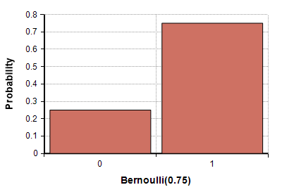
This is a discrete distribution having two possible outcomes labelled by 0 and 1 in which 1 instigates “success” with probability and 0 instigates “failure” with probability. The distribution of heads and tails in coin tossing is an example of Bernoulli with p=q= 1/2. This is the supplied discrete distribution and the building block for other more complicated discrete distributions. It has a Probability Mass Function;

• Geometric Distribution

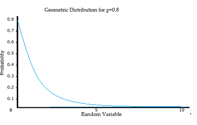
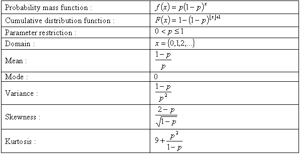
This is the probability distribution for the number of identical or independent Bernoulli trials that are done until the first success occurs. It’s a discrete distribution for n= 0,1,2 . It has the Probability Functions of

• Binomial Distribution

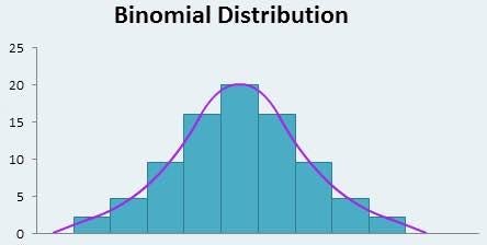
In probability theory and statistics, it has parameter n and p is the discrete probability distribution of the number of success in a sequence of n independent experiment, each asking a yes or no question. “Success”: yes/true/ one (with probability p) and “Failure”: no/false/zero (with probability q= 1-p).

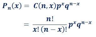
A single success or failure is a Bernoulli Trial . The model allows us to compute probability of entering a specified number of success when it’s repeated a specific number of time (e.g. in a set patients). The probability mass function is;

• Poisson Distribution

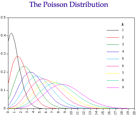
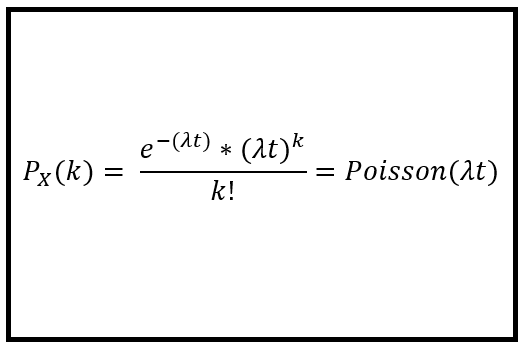
A discrete probability distribution of the number of events occuring in a given time period. It gives the average number of time the event occurs over that period. For example, a certain fast food restaurant gets an average of 3 visitors for the drive-through per minute. It is used for independent event which occur at a constant rate. Probability mass function;

Continuous Random Variables.

It has a infinite set of possible outcomes that cannot be counted. The instances are: The population of the world that’s dependent on time, rainfall in millimeters. They’re examples of Continuous Random Variables.

There are several Continuous Random Variables that are useful in probability modelling in statistics

• Uniform Distribution

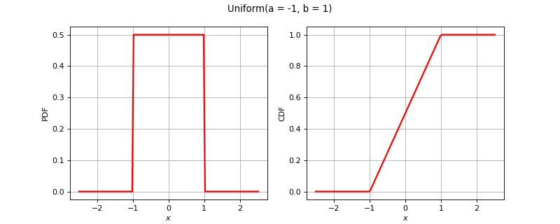
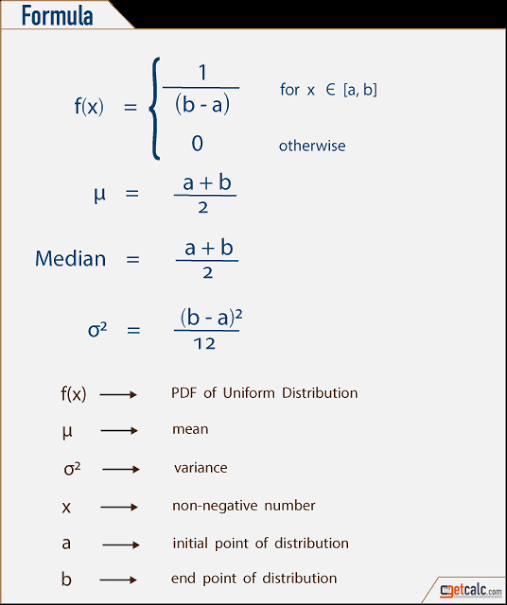
It models an experiment in which every outcome within a continuous interval is equally likely. The probability density function and cumulative distribution function for a continuous distribution on interval;

• Exponential Distribution

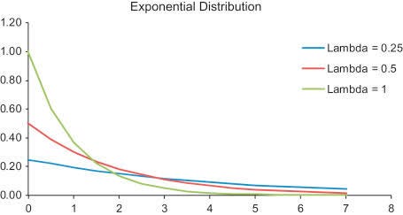
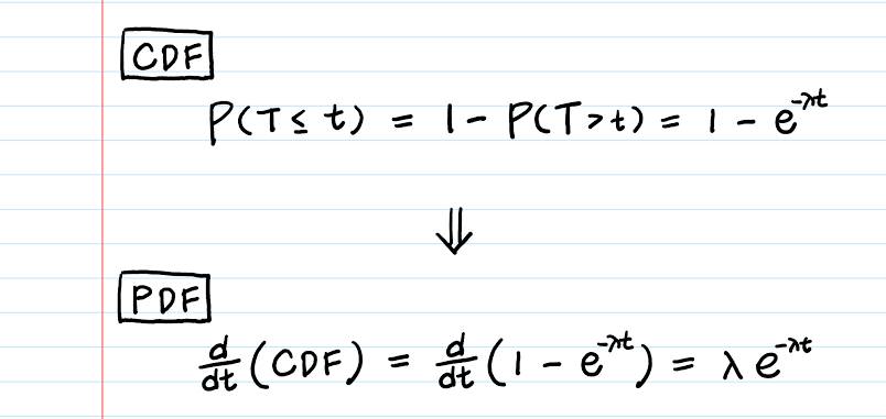
A process in which events occur continuously and independently at a constant average rate. It gives a poisson distribution with rate of change, the distribution of waiting time between successive changes. This distribution models the time that passes until a certain event occurs. E.g. decaying of radioactive particles, earthquake. Probability Density Function is the

Normal Distribution

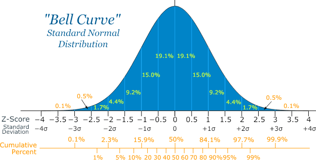
Also known as Gaussian Distribution and sometimes called “Bell Curve”. It is distribution that occurs naturally in many situations.

For example, the Bell Curve is seen in test like SAT. The bulk of students will score average (C), while the smaller number of students will score a B or D. An even smaller percentage of students score a F or an A.

The Bell Curve is symmetrical, half of the data will fall to the left of the mean; half to the right. This pattern is commonly used in business, statistics, government bodies e.t.c.

The empirical rule tells you that your data falls within certain number of Standard Deviation from the mean;

68% of the data falls within 1 Standard Deviation of the mean.

95% of the data falls within 2 Standard Deviations of the mean.

99.7% of the data falls within 3 Standard Deviations of the mean.

Properties of Normal Distribution

• The mean, median, mode are all equal.
• The curve is symmetric at the center (at mean).
• Exactly half of the values are to the left of center and exactly half of the values are to the right.
• The total area under the curve is 1.

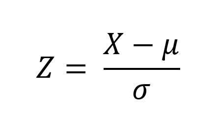
A Standard Normal Distribution is a normal distribution with a mean of 0 and standard deviation of 1 which is mostly calculated with the help of a z- score. The z-score gives an idea of how far from the mean a data point is. But technically, it’s a measure of the standard deviation below or above the population mean and raw score. The basic z-score formula is;

When analysing data such as marks achieved by 100 students for a piece of coursework. It is possible to use both descriptive and inferential statistics in your making analysis.

Descriptive Statistics

It helps describe, summarize data in a meaningful way such that patterns might emerge from the data.

Measure of Central Tendency and Speed

We can describe this central position using a number of statistics including variance, standard deviation, mean squared error, median, mean.

• Median: it’s a value repeating the higher half from the lower half of a data sample. For a dataset, it may be thought as the middle value.
• Standard Deviation: It measures the deviation of a random variable from its mean.
• Variance: The square of standard deviation.
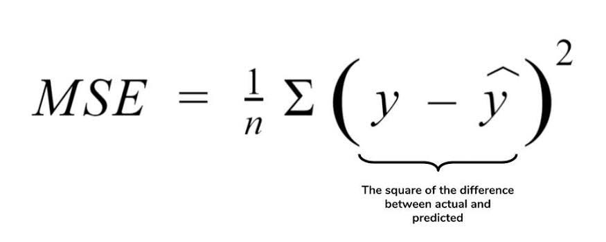
• Mean Squared Error of an estimation measures the average of the square of the errors, that is, the average squared difference between the estimated values and the actual values. MSE is a risk function. corresponding to the expected value of the squared error loss. Smaller MSE generates a better estimate at the dotplot in question.

• Expectation: Also known as the mean. Calculated by suming the probability by the events. If two observations are independent of each other and their joint expectation is supplied. We multiply their expectations together E(X Y) = EX EY. But if the two observables are not independent then we need to take their Correlation and Covariance into account.

Correlation and Covariance

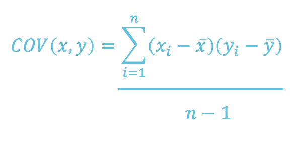
Covariance is the measure of the joint variabililty of two random variables. The metric evaluates how much and to what extent the variables change together. It’s measured in unit.

The Covariance can take negative or positive values;

Positive Covariance: It indicates that two variables tend to move in the same direction. The greater value of one variable mainly correspond to the greater value of the other variable and the same hold for the lesser value.

Negative Covariance: This regards that the two variables tend to move in reverse direction. The greater value of one variable correspond with the lesser value of the other variable. On the other hand;

Correlation: it measures the strength of the relationship between variables. It’s the scaled measure of covariance. It’s dimensionless. In other word, Correlation coefficient is always a pure value and not measured in any unit.

Non Correlation doesn’t imply independence. Correlation doesn’t mean causation.

Correlation coefficients;

“Close to 1= large positive correlation

Close to -1 = large negative correlation

Close to 0= no relationship”

Pure Value;

“P_value < 0.001 = strong certainty.

P_value < 0.05 = moderate certainty.

P_value < 0.1 = weak certainty.

P_value > 0.1 = no certainty”.

INFERENTIAL STATISTICS.

If we’re in examining the marks of 100 students, the 100 students would represent the POPULATION. Population can be small or large, as long as it includes all the data you’re interested in. Descriptive are applied to Population. Properties of population like mean, standard deviation are called parameters. However, you may not have access to the whole population you want for the whole investigation, but only a limited number of data listed. The smaller number of data gotten is called SAMPLE. Properties of samples such as mean, standard deviation are not called parameters but statistics. The graphical representation of the distribution of numerical or categorical data using bars of different heights is Histogram.

This article aims to give you a basic overview of the Probability and Statistics that you’d need on your journey to become a world-class Data Scientist. Read, Enjoy, Clap, Share or do whatever you want.